Applied Machine Learning and Predictive Modelling 1 - Notes

Author

Nils Rechberger

Published

February 9, 2026

Week 01: Linear Models

Regression

\[ y = \beta_0 + \beta_1 \cdot x_1 + \epsilon \]

\(\beta_0\) and \(\beta_1\) are the regression parameters:

\(\beta_0\) is also the intercept
\(\beta_1\) ist the slope

Coefficients

The coefficients are estimated from data. Estimated regression coefficients are denoted with a hat (e.g. \(\hat{\beta_1}\)). Fitted values (i.e. what the model predicts) are denoted with a hat as well (i.e. \(\hat{y}\)). Residuals are the difference between observed and predicted values.

\[ \text{res} = y - \hat{y} \]

If the errors are normally distributed, regression coefficients can be tested with t-tests

Caution

Dichotomising p-values into ”significant”/”non-significant” is very bad practice!

The grade of fit can be quantified with \(R^2\)

\[ R^2 = corr(y, \hat{y})^2 \]

Note: \(R^2\) is not used to formally compare model.

p-values

The p-value quantifies the probability of observing the value of the test statistic, or a more extreme value, under the null hypothesis. Low p-values are coherent with a rejection of the null hypothesis stating that there is no effect. Large p-values (close to 1) do not imply the we can accept the null hypothesis.

Testing

Categorical Values

Categorical values can be tested via F-tests by using the drop1() function or by comparing two models via the anova() function. Comparisons among levels of a factor (i.e. ”contrasts”) can be performed by using the glht() function.

Continuous or discrete variables

Continuous (and discrete) variables can be tested via F-tests (with drop1()) or by t-tests (with summary()). Sometimes the inferential results for continuous variables are best displayed and communicated with confidence intervals.

Interactions

If an interaction term is shown to be significant, then all terms involved in this interaction play a relevant role. An interaction involving two predictors is called ”two-fold interaction” (e.g. age * species)

Note: An interaction can involve more than two predictor.

Week 02: Modelling non-linearities

A Model is called to be linear if it is linear on its coeffitinents. By including polynomials (e.g. \(x_1 + {x_1}^2\)) we can model non-linear relationships with a linear model

Caution

The term “linear” here does not refer to the shape of the curve you draw in the coordinate system, but to the way the parameters (the coefficients \(\beta\)) appear in the equation.

Non-linear effect

Note

Linear models can model non-linear effects!

Non-linear models are non-linear in their coefficients.

\[ y = \beta_0 + \beta_1 \cdot x^{\beta_2} + \epsilon \]

Generalise Additive Models (GAM)

GAMs come with advantages and disadvantages compared to e.g. polynomials:

Advantages

the degree of complexity is automatically chosen
the ”estimated degrees of freedom” give the user an indication of the complexity of a given smooth term
smooth terms can be visualised

Disadvantages

GAMs can run into computational issues (e.g. models that do not converge)
the use of a quadratic term is simpler to explain than a GAM to a non-technical audience
in order to fit and understand the results of a GAM some technical knowledge is required

Week 03: Generalised Linear Models

Linear Model Assumptions

The inference on the regression coefficients (p-values and CIs) is based on the following assumption about the errors:

\[ \varepsilon \stackrel{\text{iid}}{\sim} \mathcal{N}(0, \sigma^2) \]

This means that:

The errors follow a normal distribution
The errors expected value is zero
The errors are homoscedastic (constant variance)
The errors are independent

Count Data

Below, we list a few examples of count data:

Items purchased by one client during a single shopping session.
Number of children in a family.
Faulty parts found in a car during an inspection.

Modelling count data with a linear model

If we were to use a linear model to model these data, we would assume the data to follow a normal distribution.

set.seed(1)
no.days <- 14
v.non.smoker <- c(rpois(n = no.days - 1, lambda = 0), 1)
v.smoker1_2 <- rpois(n = no.days, lambda = 5)
v.smoker.box <- rpois(n = no.days, lambda = 20)
d.smokers <- data.frame(no.cigarettes = 
                          c(v.non.smoker, v.smoker1_2, v.smoker.box),
                        person = gl(n = 3,
                                    k = no.days, 
                                    labels = c("non-smoker",
                                               "moderate smoker", 
                                               "heavy smoker")))

Note: I added a single cigarette to the non-smoker because if you don’t do so all p-values are 1

lm.smokers <- lm(no.cigarettes ~ person, data = d.smokers)
round(coef(lm.smokers), digits = 1)

          (Intercept) personmoderate smoker    personheavy smoker 
                  0.1                   5.0                  20.8

The estimates of this linear model, which assumes normality of the data, look good. Let’s dig a bit further and simulate some new observations from this linear model.

library(ggplot2)

set.seed(3)
sim.data.smokers <- simulate(lm.smokers)

ggplot(
    mapping = aes(
        y = sim.data.smokers$sim_1,
        x = d.smokers$person)) +
    geom_boxplot() +
    geom_hline(yintercept = 0) +
    ylab("simulated no. of cigarettes\n(assuming normality)") +
    xlab("person")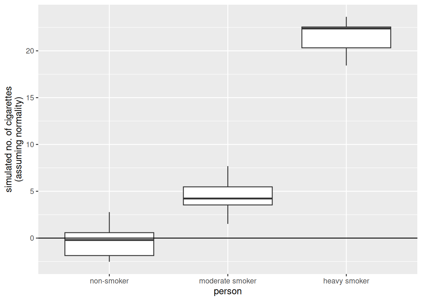

There are some striking differences between the data we simulated from the linear model and the data that made up:

The made up data are integers, the data simulated from the linear model are numeric (note that none of the simulated values is an integer).
The made up data are always larger than zero, the data simulated from the linear model go below zero as well (i.e., a negative number of cigarettes)
The variability in the made up data increases with the mean value of the person (i.e., “variability non smoker” < “variability moderate smoker” < “variability heavy smoker”). On the other hand, the variability of the simulated values is the same in all three groups.

The Poisson model

Let’s see how we could modify the linear model such that these requirements that come from the very nature of count data are fulfilled.

Avoiding negative fitted values

Consider the equation we have used so far when computing the fitted values of a linear model.

\[ \hat{y} = \hat{\beta}_0 + \hat{\beta}_1 \cdot x_1 \]

To solve the problem of negative fitted values, we must make sure that the right hand-side of this equation always produces positive results. One solution is to apply a transformation to it. For example, we can use the exponential function.

\[ \hat{y} = \exp(\hat{\beta}_0 + \hat{\beta}_1 \cdot x_1) \]

Note: Ee can rewrite the above equation by taking the logarithm on both sides.

Integers and non-constant variance

we also need to make sure that the simulated values are integers and that the variance of the observations depends on the mean values. For count data, the classical solution is to assume the data to follow a Poisson distribution (rather than the normal distribution).

\[ \log(\hat{y}) = \hat{\beta}_0 + \hat{\beta}_1 \cdot x_1 | \hat{y} = \text{Poisson}(\lambda) \]

Note: This model fullfills all the three requirements we listed above.

As a matter of fact, for the Poisson distribution the variance of the observations linearly increases with the mean value.

Generalised Linear Models

Linear models are well suited to very many situations encountered in practice. However, they are not suited when the response variable represents:

Count data: There the Poisson Model is more adequate
Binary or binomial data: There the Binomial Model is more adequate

Both these models are an extension of the linear model These models belong to the ”class” of Generalised Linear Models GLMs generalise the linear model such that non-normal data can be analysed.

Note

Note that in practice count and binomial data are virtually always overdispersed.

The Poisson model in R

To fit a Poisson model in R we can use the glm() function, where we specify the distribution to be used. GLMs generalise the linear model in the sense that the data can follow distributions other than normal.

glm.smokers <- glm(
    no.cigarettes ~ person,
    family = "poisson", ## we specify the distribution!
    data = d.smokers
    )

Let’s simulate some data from this model.

set.seed(2)
sim.data.smokers.Poisson <- simulate(glm.smokers)

ggplot(
    mapping = aes(
        y = sim.data.smokers.Poisson$sim_1,
        x = d.smokers$person
    )
) +
geom_boxplot() +
geom_hline(yintercept = 0) +
ylab("simulated no. of cigarettes\n(assuming Poisson dist)") +
xlab("person")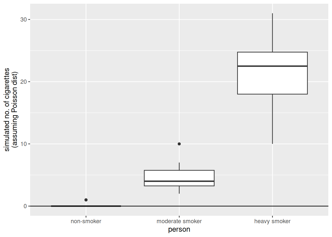

The results obtained simulating from the Poisson model are much more similar to the observations.

Binary and binomial data

Examples

Binary data (0 or 1):

Whether a client visiting a website clicks on advertisement banner.
Whether a cancer patient survived an “invasive” surgery.

Binomial data (number of success / number of trials) \(\in [0, 1]\):

The proportion of students that passes an exam (e.g., hopefully all).
The proportion of trains that gets to destination on time.

The bliss data set

library(faraway)
data(bliss)
library(dplyr)


Attaching package: 'dplyr'

The following objects are masked from 'package:stats':

    filter, lag

The following objects are masked from 'package:base':

    intersect, setdiff, setequal, union

bliss <- bliss %>%
    mutate(mortality.rate = round(dead / (dead + alive), digits = 2))

ggplot(
    data = bliss,
    mapping = aes(
        y = mortality.rate,
        x = conc
    )
) +
geom_point() +
geom_smooth(method = "lm", se = FALSE) +
ylim(0, 1) +
geom_hline(yintercept = 0:1, colour = "grey")

`geom_smooth()` using formula = 'y ~ x'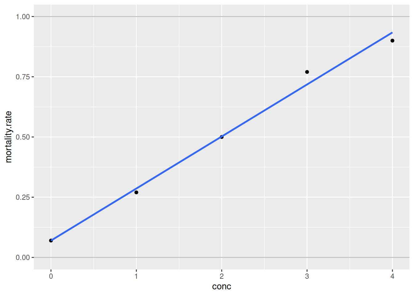

The fit seems to be fairly good. However, what problem could arise when fitting a linear model to these data?

Predictions may lay outside the probability range [0%, 100%].
Even fitted values may lay outside [0%, 100%].
Actually, the response variable is not normally distributed. Its distribution is bounded between 0% and 100%. The normal distribution is unbounded and thus inconvenient here.
The variability of the observations is not constant as it is assumed by the normal distribution. This is not evident on the graph above as there is only one observation for each concentration group. If there were many observations per group, we could see that the variability is not constant along the y-axis.

Link function for binomial data

The solution to problems 1. and 2. is to use a link function such that predictions are constrained in the [0%, 100%] range. For binary or binomial data the default choice of the link function is the “logit”.

\[ \text{logit}(y) = \log(\dfrac{y}{1-y}) | y \in [0, 1] \]

Once you applied the link function to the left-hand side of this equation, you can bring it to the right-hand side by taking its inverse on both sides.

\[ \hat{y} = \text{inverse.logit}(\hat{\beta}_0 + \hat{\beta}_1 \cdot x_1) \]

Note

To deal with the peculiarities of count and binomial/binary data, we use a link function and assume a distribution other than the normal. This is the essence of GLMs.

The Binomial model in R

Let’s fit a Binomial model to the bliss dataset.

glm.insects <- glm(
    cbind(dead, alive) ~ conc,
    family = "binomial",
    data = bliss
    )

Let’s visualise the results of this model.

new.data = data.frame(conc = seq(0, 5, length.out = 100))
new.data$pred.insects <- predict(glm.insects, newdata = new.data,
                                 type = "response")
##
ggplot(data = bliss,
       mapping = aes(y = mortality.rate,
                     x = conc)) + 
  ylim(0,1) +
  geom_hline(yintercept = 0:1, col = "gray") +
  ##
  ## predictions for conc 0 --> 5
  geom_point(data = new.data,
               mapping = aes(
      y = pred.insects,
      x = conc)) +
  ##
  ## actual observations
  geom_point(col = "red", 
             size = 3)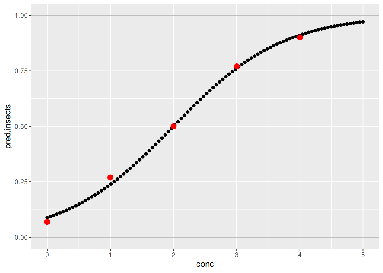

The fit of the model is quite good. Indeed, the predictions are quite close to the real observations.

Further on binary and binomial data

In many real applications there are more than two possible outcomes. Fortunately, an extension of the logistic regression to more than two classes exist. This method is called multinomial regression and is implemented in the multinom() function from the {nnet} package.

library(nnet)
multinom.iris <- multinom(
    Species ~ Sepal.Length + Petal.Width,
    trace = FALSE,
    data = iris)

Estimating the performance of a binary model

A very common way to estimate the performance of a binary model is too look at predicted values and compare them with the actual observations.

d.stab <- read.table(
    "/home/nils/dev/mscids-notes/fs26/mpm1/data/stability.dat",
    stringsAsFactors = TRUE,
    header = TRUE
)

str(d.stab)

'data.frame':   27 obs. of  2 variables:
 $ perform  : num  0 0 0 1 1 0 0 1 1 1 ...
 $ stability: num  474 432 453 481 619 584 399 582 638 624 ...

ggplot(
    data = d.stab,
    mapping = aes(
        y = perform,
    x = stability
    )
) +
geom_point()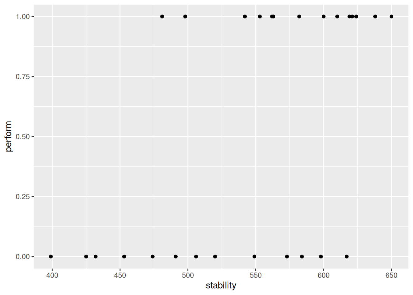

There are only two possible outcomes here: success or failure. Let’s fit a logistic regression model and add the fit to the this graph.

ggplot(
    data = d.stab,
    mapping = aes(
        y = perform,
        x = stability
    )
) + 
geom_point() +
geom_smooth(
    method = "glm", 
    se = FALSE,
    method.args = list(family = "binomial")
)

`geom_smooth()` using formula = 'y ~ x'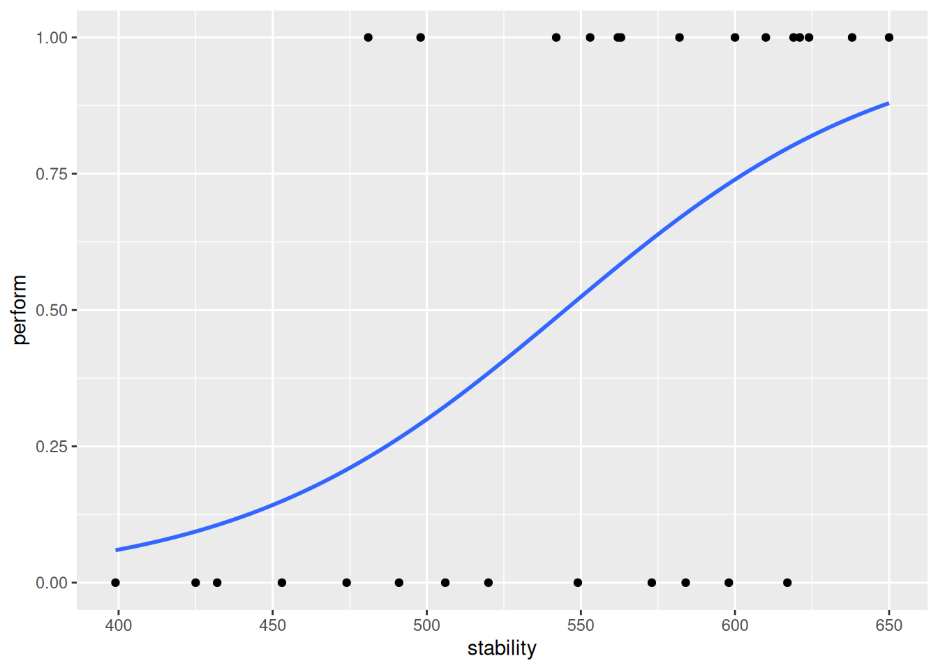

As expected, stability has a positive effect on the response variable. Let’s have a look at the fitted values for this model.

glm.stab <- glm(
    perform ~ stability,
    data = d.stab,
    family = "binomial")

fitted(glm.stab) %>% 
    round(digits = 2)

   1    2    3    4    5    6    7    8    9   10   11   12   13   14   15   16 
0.21 0.11 0.15 0.23 0.80 0.68 0.06 0.67 0.85 0.82 0.49 0.88 0.54 0.09 0.58 0.52 
  17   18   19   20   21   22   23   24   25   26   27 
0.29 0.38 0.77 0.73 0.27 0.80 0.81 0.63 0.58 0.32 0.74

Note: They are probabilities, thus, bounded within 0 and 1.

To compare the fitted values with the observed values, which are indeed binary (0 or 1), we can also discretise/dichotomise the fitted values into 0 and 1. In order to do that, we use a cutoff of 0.5. Finally, let’s compare the observed and fitted values.

fitted.stab.disc <- ifelse(
    fitted(glm.stab) < 0.5,
    yes = 0,
    no = 1
    )

d.obs.fit.stab <- data.frame(
    obs = d.stab$perform,
    fitted = fitted.stab.disc)
    
table(
    obs = d.obs.fit.stab$obs,
    fit = d.obs.fit.stab$fitted)

The diagonal entries of this matrix represent correctly labelled observations

Week 04: Support Vector Machines

What is an SVM?

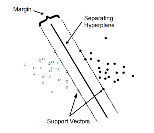
Support-vector machines (SVMs, also support-vector networks) are supervised learning models with associated learning algorithms that analyze data used for classification and regression analysis. An SVM model is a representation of the examples as points in space, mapped so that the examples of the separate categories are divided by a clear gap that is as wide as possible.

set.seed(123)

library(tidyverse)

── Attaching core tidyverse packages ──────────────────────── tidyverse 2.0.0 ──
✔ forcats   1.0.1     ✔ stringr   1.6.0
✔ lubridate 1.9.4     ✔ tibble    3.3.1
✔ purrr     1.2.1     ✔ tidyr     1.3.2
✔ readr     2.1.6     
── Conflicts ────────────────────────────────────────── tidyverse_conflicts() ──
✖ purrr::%||%()   masks base::%||%()
✖ dplyr::filter() masks stats::filter()
✖ dplyr::lag()    masks stats::lag()
ℹ Use the conflicted package (<http://conflicted.r-lib.org/>) to force all conflicts to become errors

library(e1071)


Attaching package: 'e1071'

The following object is masked from 'package:ggplot2':

    element

library(caret)

Loading required package: lattice

Attaching package: 'lattice'

The following object is masked from 'package:faraway':

    melanoma


Attaching package: 'caret'

The following object is masked from 'package:purrr':

    lift

# Load data
data(iris)

# Prepare the Data for Training
indices <- createDataPartition(iris$Species, p=.85, list = F)
train <- iris %>%
    slice(indices)

Warning: Slicing with a 1-column matrix was deprecated in dplyr 1.1.0.

test_in <- iris %>%
    slice(-indices) %>%
    select(-Species)

test_truth <- iris %>%
    slice(-indices) %>%
    pull(Species)

# Train the Support Vector Machine
iris_svm <- svm(Species ~ ., train, kernel = "linear", scale = TRUE, cost = 10)
plot(iris_svm, train, Petal.Length ~ Petal.Width)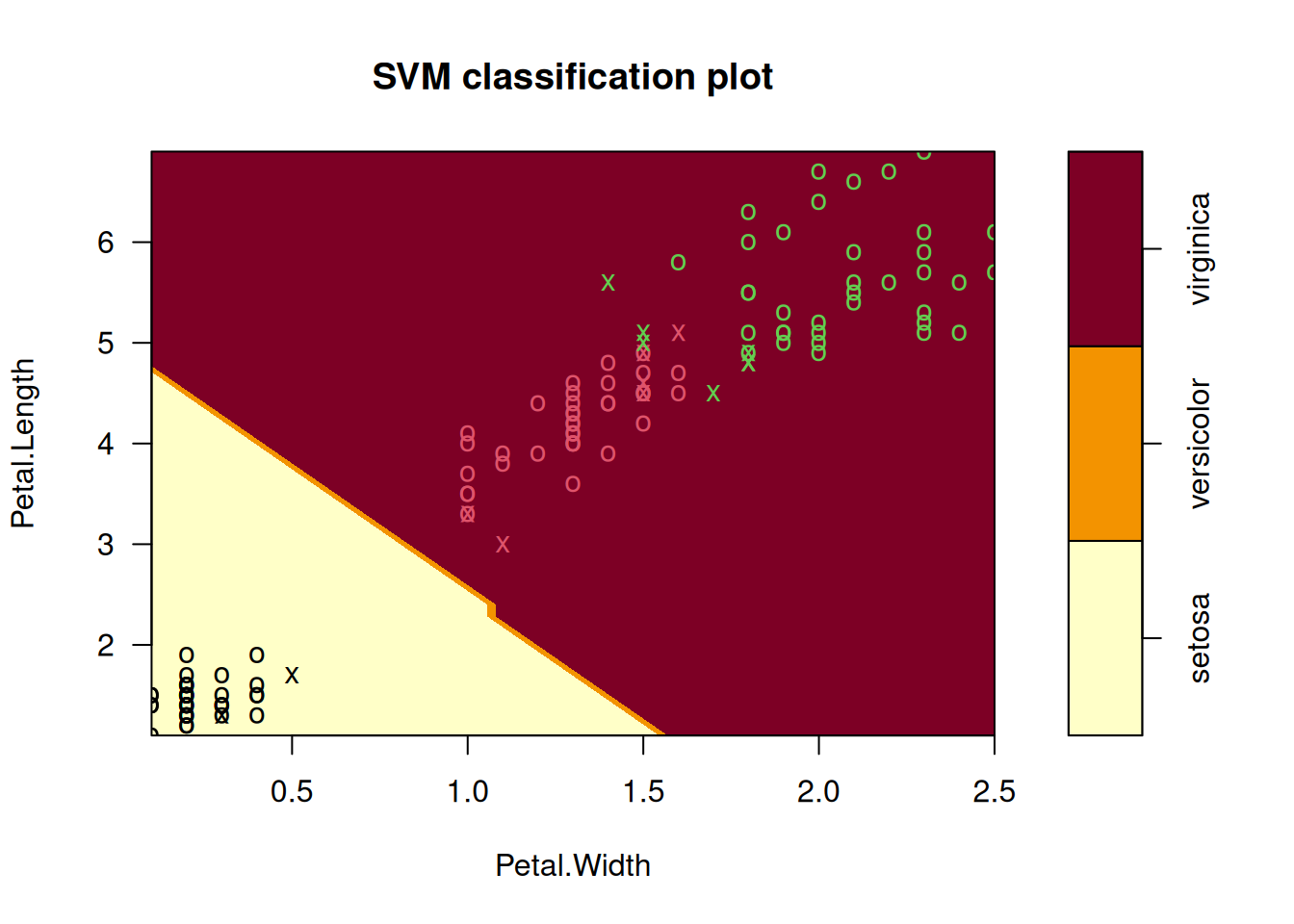

SVM Kernel Functions

In many real-world scenarios, data is non-linearly separable. A standard linear SVM would fail here. Instead of manually performing complex mathematical transformations to move data into a higher dimension (which is computationally expensive), we use the Kernel Trick. A kernel function calculates the “similarity” or “inner product” between two points in a high-dimensional space without actually transforming the data points themselves.

Soft Margin Formulation

If you try to force a Hard Margin SVM to separate every single point perfectly, you often end up with overfitting or a model that simply fails to find a solution because the data overlaps.

The Soft Margin Formulation was introduced to solve this by allowing the SVM to make a few “mistakes” for the sake of a better, more general boundary.

The Role of the Hyperparameter \(C\)

The variable \(C\) is the most important dial you can turn. it controls the trade-off between “smoothness” and “accuracy.”

Analyse Model Performance

test_pred <- predict(iris_svm, test_in)
table(test_pred)

test_pred
    setosa versicolor  virginica 
         7          6          8

conf_matrix <- confusionMatrix(test_pred, test_truth)
conf_matrix

Confusion Matrix and Statistics

            Reference
Prediction   setosa versicolor virginica
  setosa          7          0         0
  versicolor      0          6         0
  virginica       0          1         7

Overall Statistics
                                          
               Accuracy : 0.9524          
                 95% CI : (0.7618, 0.9988)
    No Information Rate : 0.3333          
    P-Value [Acc > NIR] : 4.111e-09       
                                          
                  Kappa : 0.9286          
                                          
 Mcnemar's Test P-Value : NA              

Statistics by Class:

                     Class: setosa Class: versicolor Class: virginica
Sensitivity                 1.0000            0.8571           1.0000
Specificity                 1.0000            1.0000           0.9286
Pos Pred Value              1.0000            1.0000           0.8750
Neg Pred Value              1.0000            0.9333           1.0000
Prevalence                  0.3333            0.3333           0.3333
Detection Rate              0.3333            0.2857           0.3333
Detection Prevalence        0.3333            0.2857           0.3810
Balanced Accuracy           1.0000            0.9286           0.9643

Pros & Cons of SVM

Pros

It works really well with a clear margin of separation
It is effective in high dimensional spaces
It is effective in cases where the number of dimensions is greater than the number of samples
It uses a subset of training points in the decision function (support vectors), so it is memory efficient

Cons

It is not always straightforward to scale the different variables “equally”
It is very prone to overfitting (different Kernel functions, hyperparameters etc.)
It doesn’t perform well when we have large data set because the required training time is higher
It also doesn’t perform very well, when the data set has more noise i.e. target classes are overlapping
It doesn’t directly provide probability estimates

Support Vector Regression

SVR gives us the flexibility to define how much error is acceptable in our model and will find an appropriate line (or hyperplane in higher dimensions) to fit the data. In contrast to OLS, the objective function of SVR is to minimize the coefficients not the squared error.

Summary

Support Vector Machine (SVM) is a non-probabilistic binary linear classifier
It can handle non-linear boundaries with the Kernel function/trick
It can be extended to more than two classes as well
It is also possible to do regression using this technique (Support Vector Regression)
Particularly useful in cases where we want to ignore errors up to a certain tolerance
Be careful with scaling your data and overfitting!

Week 05: Model Validation

The validation should simulate the setting in which the model is used. The choice of the most suited method depends on the situation. ften several methods are used simultaneously (to compare results).

The best model is the most useful one!

Data Set Approaches

Validation Set Approach

A set of \(n\) observations is randomly split into training and validation sets. The statistical learning method is then fitted to the training set and its performance evaluated on the validation set.

set.seed(1)

df <- data.frame(
  x = 1:100,
  y = (1:100) * 2 + rnorm(100)
)

n <- nrow(df)

train_size <- floor(0.7 * n)
train_indices <- sample(seq_len(n), size = train_size)

train_set <- df[train_indices, ]
test_set  <- df[-train_indices, ]

train_set

    x          y
77 77 153.556708
90 90 180.267099
98 98 195.426735
66 66 132.188792
19 19  38.821221
17 17  33.983810
34 34  67.946195
75 75 148.746367
31 31  63.358680
35 35  68.622940
46 46  91.292505
96 96 192.558486
93 93 187.160403
16 16  31.955066
40 40  80.763176
9   9  18.575781
50 50 100.881108
24 24  46.010648
10 10  19.694612
79 79 158.074341
32 32  63.897212
39 39  79.100025
37 37  73.605710
12 12  24.389843
14 14  25.785300
87 87 175.063100
15 15  31.124931
2   2   4.183643
65 65 129.256727
67 67 132.195041
95 95 191.586833
5   5  10.329508
41 41  81.835476
92 92 185.207868
36 36  71.585005
49 49  97.887654
68 68 137.465555
29 29  57.521850
21 21  42.918977
1   1   1.373546
53 53 106.341120
20 20  40.593901
42 42  83.746638
99 99 196.775387
58 58 114.955865
83 83 167.178087
60 60 119.864945
54 54 106.870637
22 22  44.782136
38 38  75.940687
84 84 166.476433
88 88 175.695816
30 30  60.417942
63 63 126.689739
73 73 146.610726
8   8  16.738325
76 76 152.291446
97 97 192.723408
26 26  51.943871
86 86 172.332950
78 78 156.001105
45 45  89.311244
7   7  14.487429
43 43  86.696963
64 64 128.028002
85 85 170.593946
27 27  53.844204
74 74 147.065902
25 25  50.619826
6   6  11.179532

5-fold CV

A set of \(n\) observations is randomly divided into five non-overlapping groups. Each of these fifths acts as a validation set and the remainder as a training set. The test error is estimated by averaging the five resulting mean squared error (MSE) estimates.

set.seed(1)
df <- data.frame(x = 1:100, y = rnorm(100))

df <- df[sample(nrow(df)), ]

folds <- cut(seq(1, nrow(df)), breaks = 5, labels = FALSE)

test_indices <- which(folds == 1)
test_data  <- df[test_indices, ]
train_data <- df[-test_indices, ]

train_data

      x            y
32   32 -0.102787727
39   39  1.100025372
37   37 -0.394289954
12   12  0.389843236
14   14 -2.214699887
87   87  1.063099837
15   15  1.124930918
2     2  0.183643324
65   65 -0.743273209
67   67 -1.804958629
95   95  1.586833455
5     5  0.329507772
41   41 -0.164523596
92   92  1.207867806
36   36 -0.414994563
49   49 -0.112346212
68   68  1.465554862
29   29 -0.478150055
21   21  0.918977372
1     1 -0.626453811
53   53  0.341119691
20   20  0.593901321
42   42 -0.253361680
99   99 -1.224612615
58   58 -1.044134626
83   83  1.178086997
60   60 -0.135054604
54   54 -1.129363096
22   22  0.782136301
38   38 -0.059313397
84   84 -1.523566800
88   88 -0.304183924
30   30  0.417941560
63   63  0.689739362
73   73  0.610726353
8     8  0.738324705
76   76  0.291446236
97   97 -1.276592208
26   26 -0.056128740
86   86  0.332950371
78   78  0.001105352
45   45 -0.688755695
7     7  0.487429052
43   43  0.696963375
64   64  0.028002159
85   85  0.593946188
27   27 -0.155795507
74   74 -0.934097632
25   25  0.619825748
6     6 -0.820468384
48   48  0.768532925
71   71  0.475509529
4     4  1.595280802
3     3 -0.835628612
94   94  0.700213650
13   13 -0.621240581
91   91 -0.542520031
51   51  0.398105880
44   44  0.556663199
69   69  0.153253338
23   23  0.074564983
82   82 -0.135178615
81   81 -0.568668733
61   61  2.401617761
100 100 -0.473400636
52   52 -0.612026393
72   72 -0.709946431
80   80 -0.589520946
33   33  0.387671612
89   89  0.370018810
57   57 -0.367221476
70   70  2.172611670
55   55  1.433023702
28   28 -1.470752384
59   59  0.569719627
62   62 -0.039240003
18   18  0.943836211
11   11  1.511781168
47   47  0.364581962
56   56  1.980399899

Leave one out CV (LOOCV)

A set of \(n\) data points is repeatedly split into a training set containing all but one observation and a validation set containing only that observation. The test error is estimated by averaging the resulting MSE’s.

set.seed(1)

df <- data.frame(x = 1:100, y = rnorm(100))
n  <- nrow(df)

predictions <- numeric(n)

# The LOOCV Loop
for (i in 1:n) {
  train_data <- df[-i, ]
  test_data  <- df[i, ]
  
  model <- lm(y ~ x, data = train_data)

  predictions[i] <- predict(model, test_data)
}

mse_loocv <- mean((df$y - predictions)^2)
mse_loocv

[1] 0.8317288

Week 06: Artificial Neural Networks

Artificial neural networks (ANNs), usually simply called neural networks (NNs), are computing systems vaguely inspired by the biological neural networks that constitute animal brains. An ANN is based on a collection of connected units or nodes called artificial neurons, which loosely model the neurons in a biological brain. Each connection, like the synapses in a biological brain, can transmit a signal to other neurons. An artificial neuron that receives a signal then processes it and can signal neurons connected to it.

Motivation & History

Model a program that works similar to the Human Brain. Build of different neurons (up to \(10^9\)). Type and strength of connection influence the flow of the signals.

The Perceptron

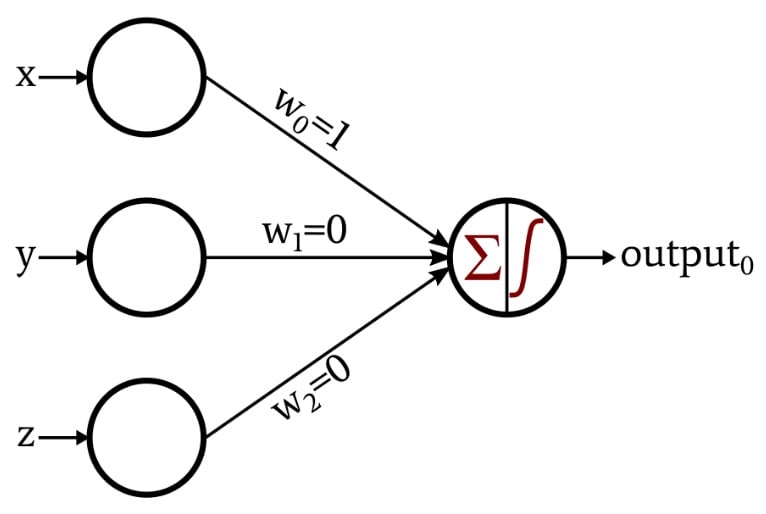
A Perceptron is an algorithm for supervised learning of binary classifiers. It mimics a single biological neuron by receiving multiple signals, processing them, and deciding whether or not to “fire” an output.

Input Values (\(x_n\)): These are the features of your data (e.g., pixels in an image or dimensions of a fruit).
Weights (\(w_n\)): Each input is assigned a weight that represents its importance. The network “learns” by adjusting these weights.
Summation Function: The Perceptron calculates the weighted sum of the inputs and adds a bias (\(b\)). The bias allows the model to shift the activation function up or down.

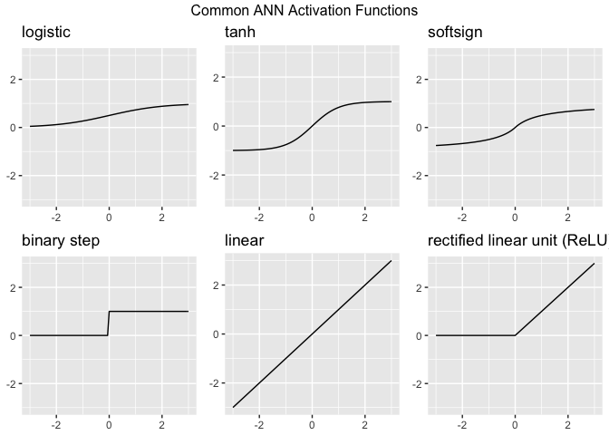
Activation Functions

Activation functions are the “gatekeepers” of a neural network. While the Perceptron uses a simple step function, modern Artificial Neural Networks (ANNs) use more complex functions to help the model learn intricate patterns. Without an activation function, a neural network is just a giant linear regression model—no matter how many layers you add, it could only represent linear relationships. Activation functions introduce non-linearity, allowing the network to learn “curvy” and complex boundaries.

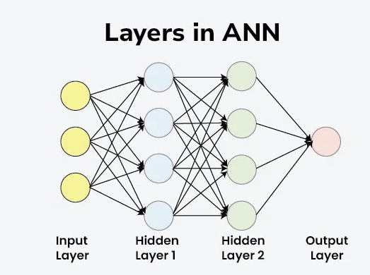
Layers

Layers are the structural building blocks that organize how data is processed. Instead of just one neuron (like the Perceptron), we stack them to create “Deep” networks. Think of layers as a filtration system: each layer extracts more complex features from the raw data until the final layer can make a confident prediction.

Input Layer: Receive data
Hidden Layer: Feature extraction & pattern recognition
Output Layer: Final prediction / Classification

Note

As you add more hidden layers, it becomes harder for humans to understand exactly why a network made a specific decision. This is why deep learning is often referred to as a “black box.”

Gradient Descent

Gradient Descent is an iterative optimization algorithm used to find the minimum of a function. In the context of ANNs, that function is the Loss Function (the measure of how “wrong” the model’s predictions are).

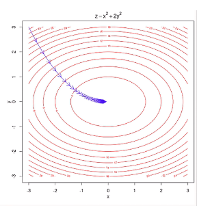
Learning Rate

The size of the “steps” you take down the mountain is controlled by the Learning Rate. This is a crucial “hyperparameter” you set before training.

Too High: You might overstep the valley and bounce back and forth, never reaching the bottom.
Too Low: It will take forever to reach the bottom, and you might get stuck in a “Local Minimum” (a small dip that isn’t the true lowest point).

Deep Learning

Deep learning is essentially the “heavy lifting” department of Artificial Intelligence. While traditional AI relies on human-coded rules, deep learning uses Artificial Neural Networks to mimic how the human brain processes information.

Neural networks have been around since the 1950s, but they only took off recently because of two main things: Big Data (the internet provided the “textbooks” for these models) and GPU Computing (video game hardware turned out to be perfect for the complex math required).

Note: Deep Learning is just Classical Network with many hidden layers (deep).

Generative Adversial Networks (GANs)

Generative Adversarial Networks, or GANs, are a fascinating architecture in deep learning where two neural networks “fight” each other to create incredibly realistic data, such as images, music, or speech. A GAN consists of two distinct models that are trained simultaneously:

The Generator (The Forger): Its job is to create fake data that looks real. It starts by producing random noise but learns over time which features make an image look “authentic.”
The Discriminator (The Detective): Its job is to look at a piece of data and decide if it is “Real” (from the actual training set) or “Fake” (created by the Generator).

Week 07 - General Topics

Parametric vs. non-parametric models

Parametric Models

The word “parametric” refers to a fixed set of parameters. Before looking at any data, you decide on a specific mathematical “shape” (like a straight line). No matter how much data you throw at it, the number of parameters remains constant (e.g., just a slope and an intercept).

Non-parametric Models

The name is a bit of a misnomer—it doesn’t mean “zero parameters.” Instead, it means the number of parameters is not predetermined. The model structure grows and changes based on the data. The “parameters” are often the data points themselves or an ever-expanding set of branches and nodes.

Comparison

Feature	Parametric Models (e.g., LM, GLM)	Non-parametric Models (e.g., Random Forest, NN)
Model Structure	Fixed / Predefined (e.g., a linear equation).	Flexible / Learns the shape from the data.
Parameter Count	Fixed (does not change with more data).	Grows (more data = more complex structure).
Primary Goal	Inference: Understanding the “why” and testing hypotheses.	Prediction: Achieving the highest accuracy possible.
Data Requirements	Works well with small datasets.	Usually requires large amounts of data.
Complexity	Simple, easy to interpret (“Glass Box”).	Complex, harder to explain (“Black Box”).
Assumptions	Strong assumptions (e.g., normality, linearity).	Minimal assumptions about the data distribution.