tRange<-1:40
Xt<-cos(2*pi/10*tRange)+runif(40)
plot(Xt,type="o")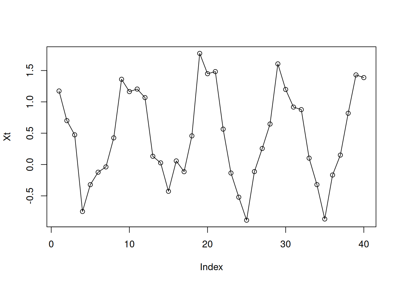
Coming soon…
Instead of the original time series 𝑋𝑡, consider the log-transformed time series with the elements.
\[ g_t = \log({X_t}) \]
When to apply it?:
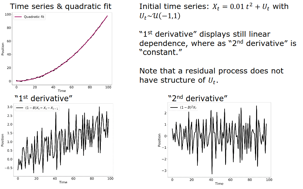
Let’s take a linear function (defined on a set of integer numbers)
\[ X_t = m \cdot t + b \]
Then, the backward difference
\[ X_t - X_{t-1} = (m \cdot t + b) - (m \cdot (t-1) + b) = m \]

Use multiple derivatives to eliminate lower-order terms. Trend order is reduced, but the stationary part may be more complex. After trend is eliminated, maybe a new dependencies in the stationary part.
Seasonality manifests itself by a repetitive behavior after a fixed lag time \(p\).
tRange<-1:40
Xt<-cos(2*pi/10*tRange)+runif(40)
plot(Xt,type="o")
What happens if we differentiate now with lag 10?
plot(diff(Xt,10),type="o")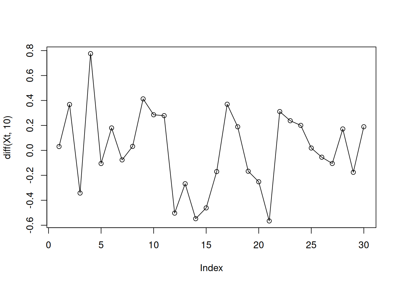
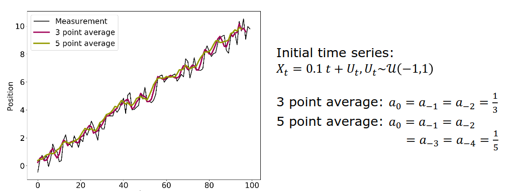
To reduce the noise element in an experiment, you can repeat the measurement multiple times and then calculate the average.
set.seed(42)
Xt<-5+runif(50)
plot(Xt,type="o")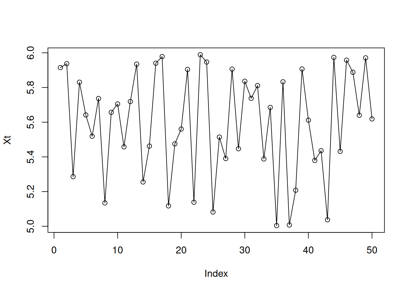
filtered<-filter(Xt,filter=rep(1,10)/10)
plot(Xt)
points(filtered,type="l")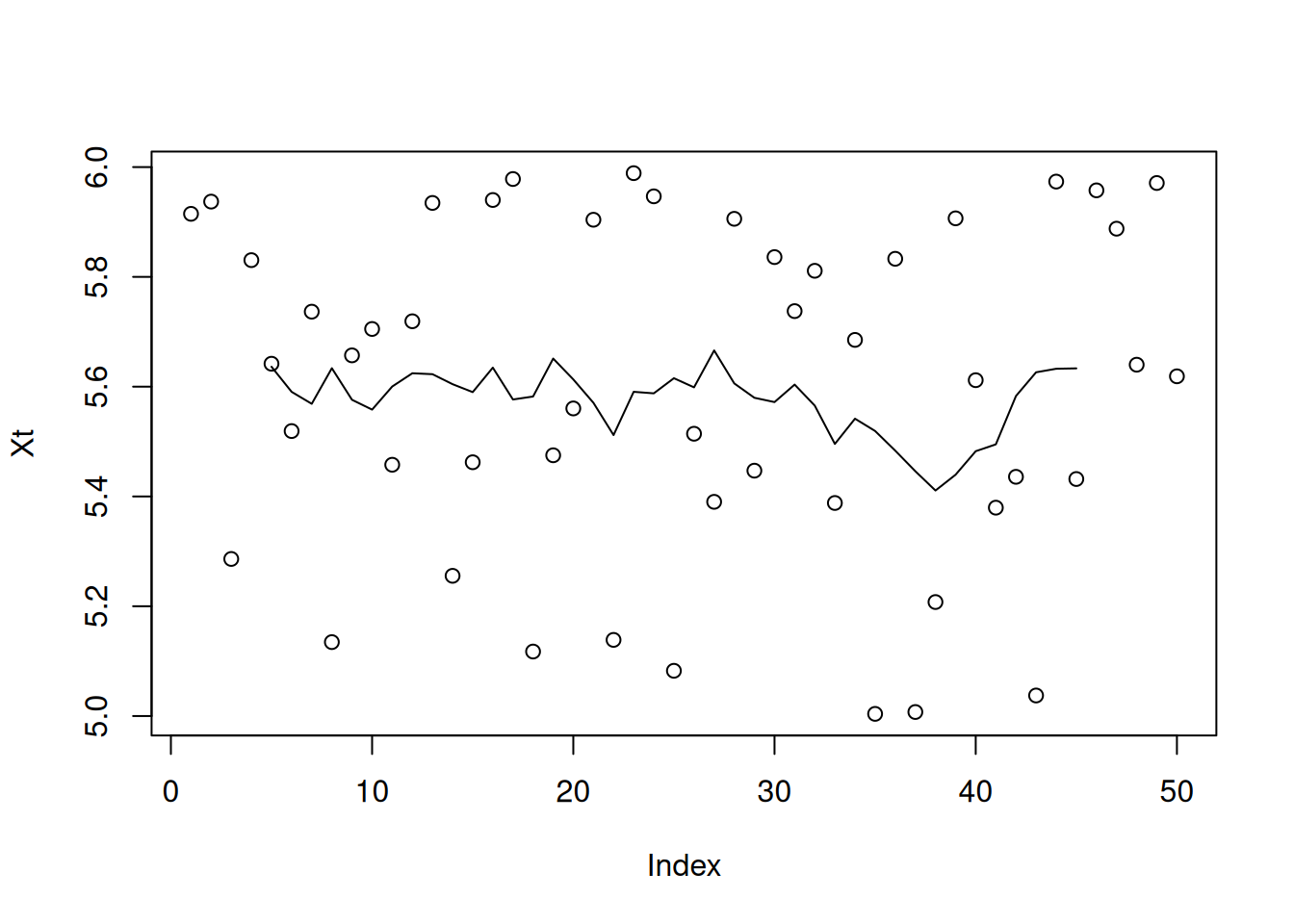
By averaging measurements, we obtain a new averaged time series. By increasing the number of averaged measurements, the parts converges to the expectation value of the measurement error, i.e. 0.
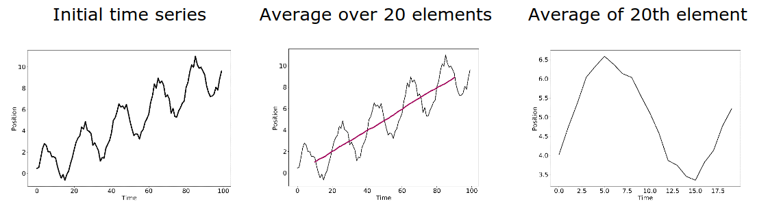
Note: The short-term variations are smoothed out and the trend is confirmed.
In case of seasonality effects, the filter has to expand over the full period to extract the trend. To quantify the seasonal impact, the values of the same time in the season have to be averaged.
Linear filters are great if periodicity is obvious; but in less obvious cases, extracting the individual components may be laborious. An alternative is the seasonal-trend decomposition procedure by Loess: An iterative, non-parametric smoothing algorithm that is more robust.
If you know the generative model, you can use fitting to determine the contributions of trend and seasonality. Fitting methods (among others):
set.seed(42)
#Generate the sample data set
t<-seq(1,100,length=100)
data<-0.1*t+cos(2*pi/10*t)+runif(100)
ts<-ts(data)
#Fit the model
fit<-lm(ts~t+cos(2*pi/10*t))
summary(fit)
Call:
lm(formula = ts ~ t + cos(2 * pi/10 * t))

Residuals:
     Min       1Q   Median       3Q      Max
-0.58266 -0.22271  0.04478  0.25411  0.49285

Coefficients:
                   Estimate Std. Error t value Pr(>|t|)
(Intercept)        0.639744   0.059840   10.69   <2e-16 ***
t                  0.097718   0.001029   94.98   <2e-16 ***
cos(2 * pi/10 * t) 0.973247   0.041999   23.17   <2e-16 ***
---
Signif. codes:  0 '***' 0.001 '**' 0.01 '*' 0.05 '.' 0.1 ' ' 1

Residual standard error: 0.2969 on 97 degrees of freedom
Multiple R-squared:  0.9901,    Adjusted R-squared:  0.9899
F-statistic: 4836 on 2 and 97 DF, p-value: < 2.2e-16The autocorrelation depends only on the lag 𝑘 for weakly or strongly stationary time series.
\[ p(k) := Cor(X_{t+k}, X_t) \]
The correlation \(p(k)^2\) squared corresponds to the percentage of variability explained by the linear association between \(X_t\) and \(X_{t+k}\).
Exchange average over realizations with average over time.
address <- "https://raw.githubusercontent.com/AtefOuni/ts/master/Data/wave.dat"
dat <- read.table(address,header=T)

#Generate ts object
wave<-ts(dat$waveht)

#Visualize the data
plot(window(wave,1,60),ylab="Height")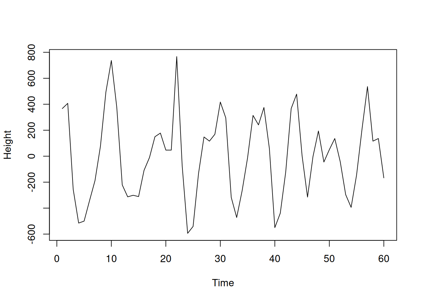
#Lag plot
lag.plot(wave,do.lines=FALSE,pch=20)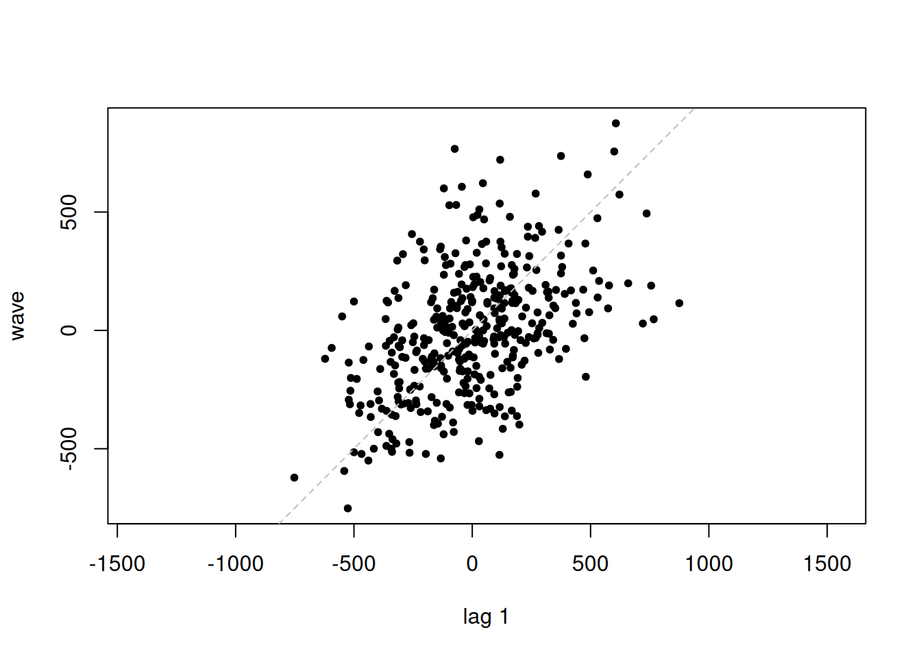
# Calculate the Pearson Correlation coefficients
n <- length(wave)
lagCorrel <- rep(0,n)

for (i in 1:(n-1)){
lagCorrel[i]=cor(wave[1:(n-i)],wave[(i+1):n])
}

plot(lagCorrel,type="l")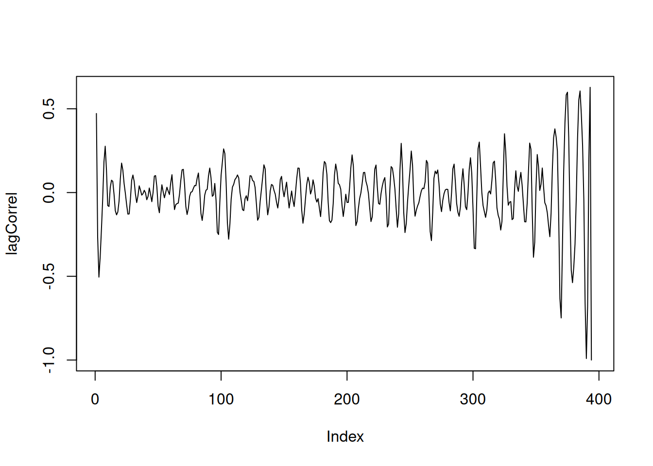
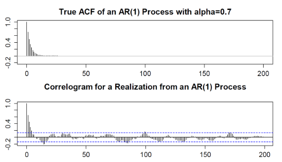
The plug-in estimator is the standard approach to computation autocorrelations. Calculated with an acf function in R.
Warning: Non-linear relations may confuse the autocorrelation.
Standard command: acf(data) for plug-in estimator values.
data(sunspot.year)
acf(sunspot.year)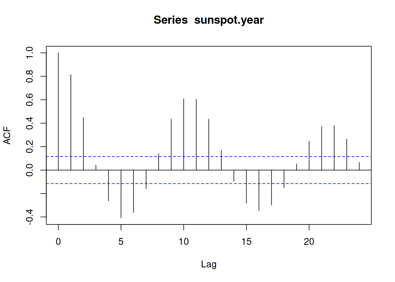
The first lag at lag \(0\) always have to be a value of \(1\)
Under the null hypothesis of a time series process with iid distributed random variables, a 95 % acceptance region for the null hypothesis is:
\[ \pm \dfrac{1.96}{\sqrt{n}} \]
For stationary processes, plug-in estimator value \(\hat{p}(k)\) within the confidence band \(\pm \frac{1.96}{\sqrt{n}}\) are considered to be different from 0 only by chance.
The Ljung-Box test assesses the null hypothesis that the random variables are independent when the \(h\) autocorrelation coefficients \(\hat{p}(k)\) for \(k = 1, \dots , h\) are equal to zero.
Box.test(sunspot.year, lag=10, type="Ljung-Box")
    Box-Ljung test

data:  sunspot.year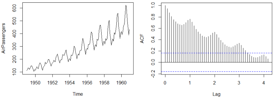
X-squared = 542.41, df = 10, p-value < 2.2e-16For non-stationary time series, the ACF decays only slowly.
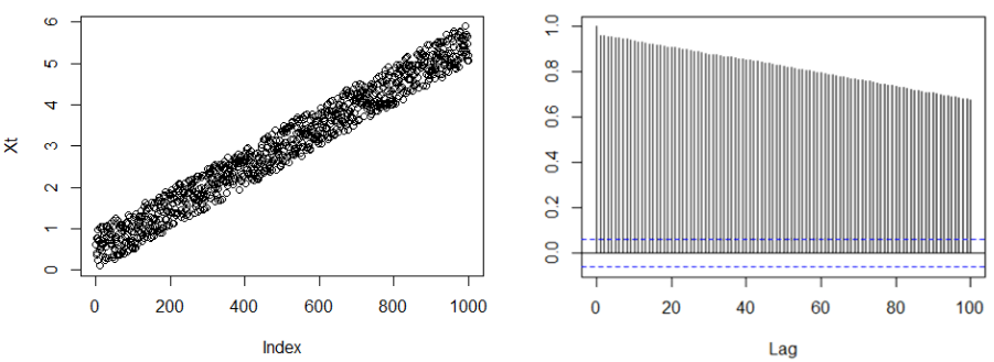
For time series with seasonality, the ACF displays periodic structure.
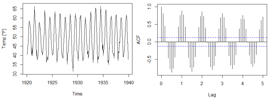
Time series with seasonality and trend, the ACF displays periodicity and slow decay.
Outliers may be diagnosed by lagged scatter plots. Note that each outlier causes other outliers.
The plug-in estimator \(\hat{p}(k)\) is sensitive to outliers.
A challenge in the interpretation of ACFs is that the effect of smaller lags remains. The partial autocorrelation function (PACF) gives the partial correlation of a stationary time series with its own lagged values, regressed the values of the time series at all shorter lags.
pacf(sunspot.year)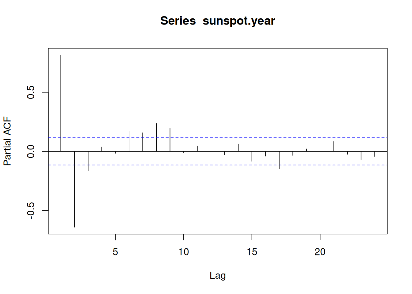
A time series process \({𝑊𝑡, 𝑡 ∈ ℕ}\) is called white noise if it is a sequence of independent and identically distributed random variables with mean \(0\).
Note: The name “white” indicates that all frequencies are included, as in the case of “white light.”
set.seed(42)
whiteNoise <- ts(rnorm(100,mean=0,sd=1))
plot(whiteNoise)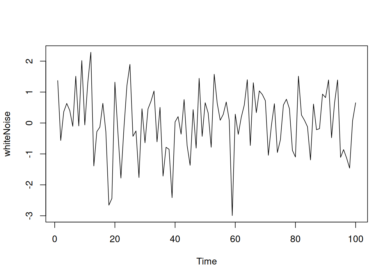
acf(whiteNoise)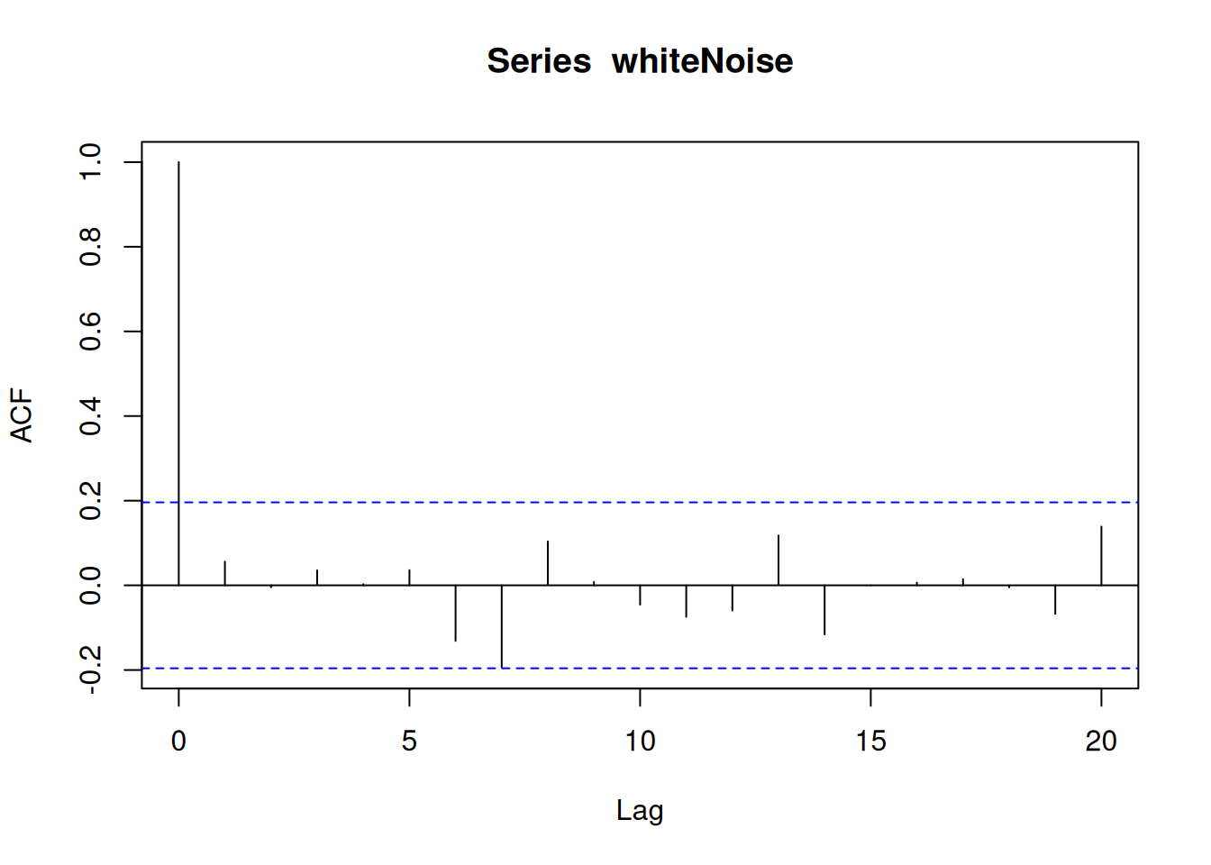
pacf(whiteNoise)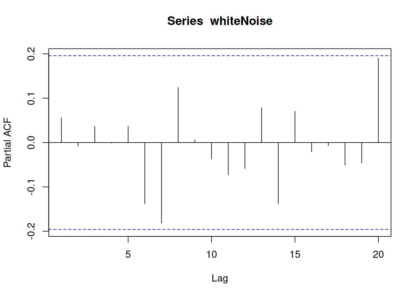
A series of \(iid\) random variables \(e_t\), which are individually independent of the proceeding time series elements \(X_t\)
The following models are often used when there is limited information about how time series data is generated:
Express the current random variable as a linear combination of the last \(p\) time steps and a “completely independent” term \(e_t\) called innovation.
\[ X_t = \alpha_1 X_{t-1} + \dots + \alpha_p X_{t-p} + e_t \]
where \(\alpha_x\) is a set of finite parameters and \(e_t\) a series of independent random variables.
Trajectory of an object moving along a line. At each moment, the object takes randomly the decision in which direction to move on.
\[ X_t = X_{t-1} + e_t \]
where \(e_t\) is random with equal probability for \(-1\) and \(1\).
set.seed(42)
step<- 1 - 2 * round(runif(100))
X_t<-cumsum(step)
plot(X_t, type="lines")
Warning in plot.xy(xy, type, ...): plot type 'lines' will be truncated to first
character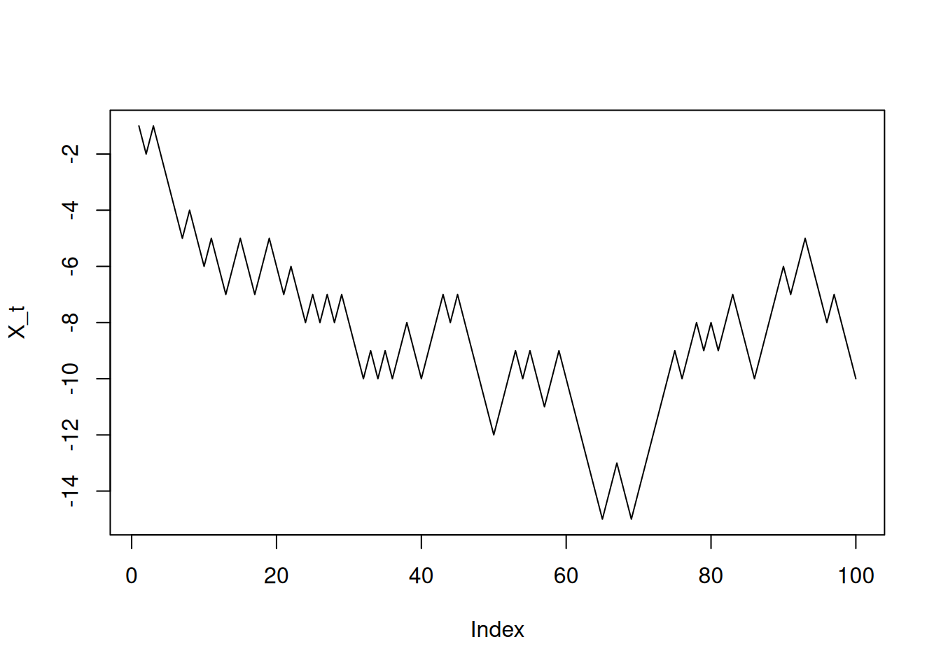
We would like to simulate:
\[ X_t = 0.5 X_{t-1} + 0.3 X_{t-2} + e_t \text{ with } e_t \sim N(0,1) \text{ iid.} \]
set.seed(42)
ar.coefficients <- c(0.5, 0.3)
simData <- arima.sim(n=1000,model=list(ar=ar.coefficients))
plot(simData)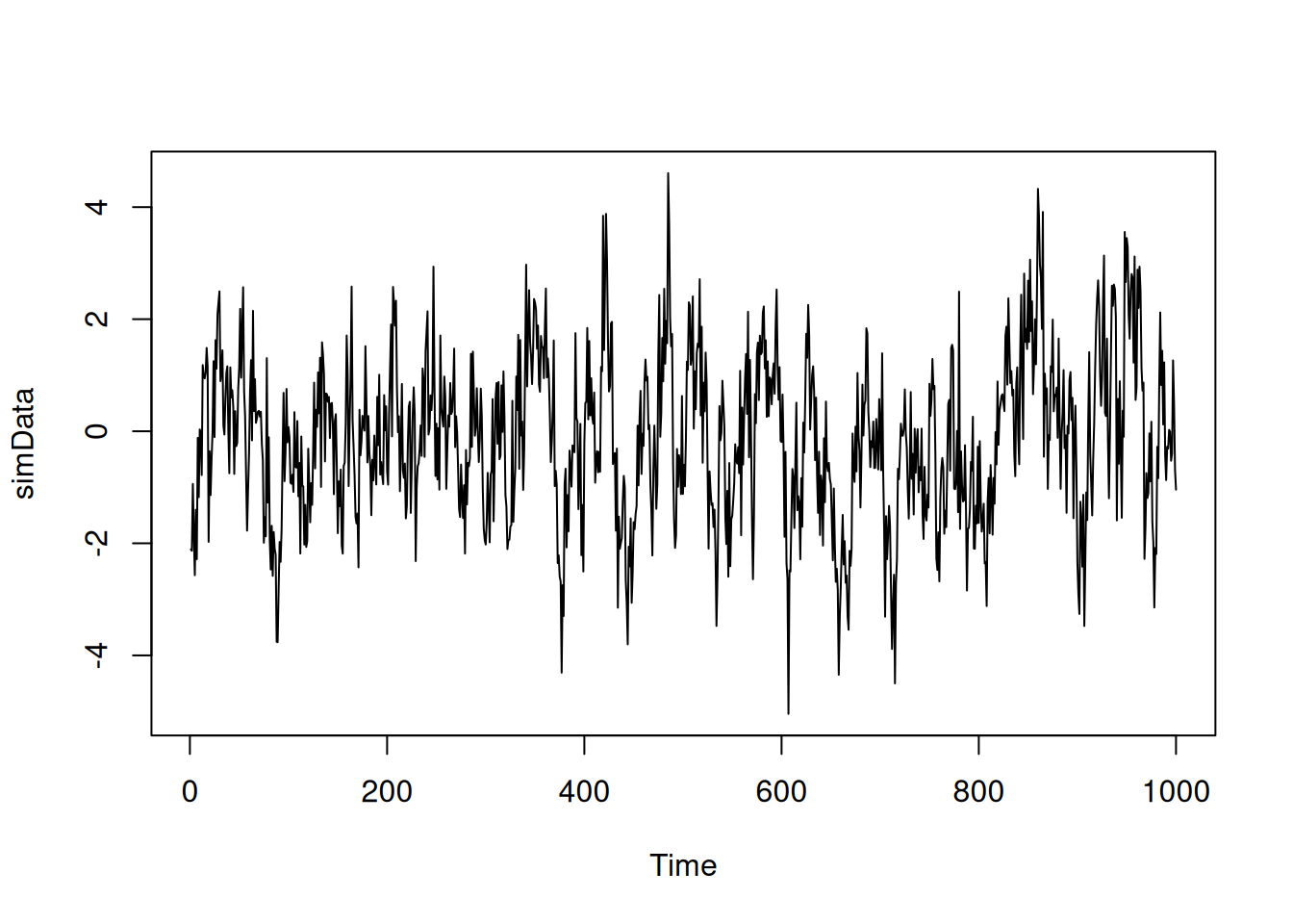
acf(simData)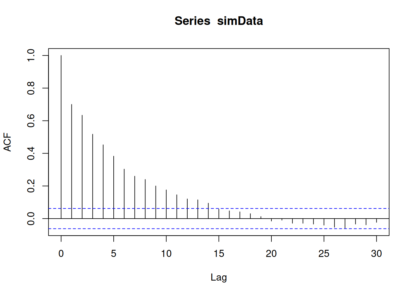
pacf(simData)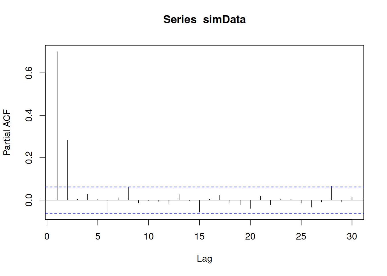
AR(p) models are stationary when the:
polyroot(c(1,-0.8,-0.4))[1] 0.8708287+0i -2.8708287+0iAs the first value has an absolute value below 1, the time series is not stationary.
The AR(1) process:
\[ X_t = 0.75 * X_t + e_t \]
is stationary because the characteristic polynomial:
polyroot(c(1,-0.75))[1] 1.333333+0iFor the model identification of AR(p) processes, two properties are key:
Try fitting an \(AR(2)\), \(AR(4)\), \(AR(7)\), \(AR(11)\)
Time series are often not centered: I.e. instead of a classical AR(p) process, a centered version has to be fitted.
\[ Y_t = m + X_t = m + \alpha_1 X_{t-1} + \dots + \alpha_p X_{t-p} + e_t \]
Fitting parameters are: - the global mean \(m\) - the AR-coefficients \(\alpha_1, \dots, \alpha_p\) - the parameters defining the distribution of the innovation \(e_t\). Here, we assume a normal distribution.
We want to estimate the parameters from the model equation, we have a total od \(n-p\) points for this, because we have a total of \(n\) time segments and each equation links \(p\) time instance.
The OLS procedure is:
ar.ols(data,order=p)Basic idea: The model coefficients and the ACF values are entangled. The values of the auto-correlation function depend on the model coefficients. A careful calculation for an AR(p) model yields the following equations, called Yule-Walker equations:
\[ \sum_{i=1}^{p} \alpha_i \rho(k-i) = \rho(k) \quad \text{for } k > 0 \]
\[ \sum_{i=1}^{p} \alpha_i \rho(i) = \rho(0) - \sigma_{E}^{2} \quad \text{for } k = 0 \]
Note: Note that the autocorrelation function is symmetric, i.e. \(p(-k) = p(k)\) for all \(k\).
To fit the AR(p) model parameters, we must solve the above equations with the estimated values of the auto correlation function.
ar.yw(data,order=p)Offers another fitting cost function that exploit also the first \(p\) function values.
ar.burg(data,order.max=p)Determines the parameter based on an optimization of the maximum likelihood function
arima(Data,order=c(2,0,0))One option is to use the Akaike information criterion (AIC), which estimates the relative amount of information lost by the considered model. The less information a model loses, the higher the quality of that model.
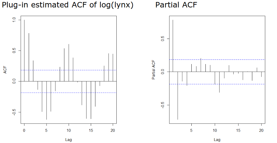
f.burg<-ar.burg(log(lynx))
plot(
    0:f.burg$order.max,
    f.burg$aic,
    type="l"
    )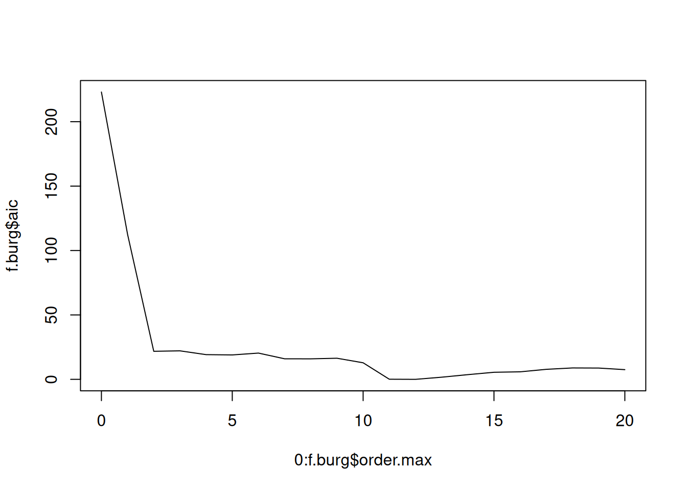
Note: No order parameter is given any more.
# Fitting the two models
fit.2<-arima(log(lynx),order=c(2,0,0))
fit.11<-arima(log(lynx),order=c(11,0,0))

# Display the time series and model predictions
plot(log(lynx))
lines(log(lynx) - fit.2$resid, col = "red")
lines(log(lynx) - fit.11$resid, col = "blue")
legend("topleft",
       legend = c("AR(2)", "AR(11)"),
       col = c("red", "blue"),
       lty = 1)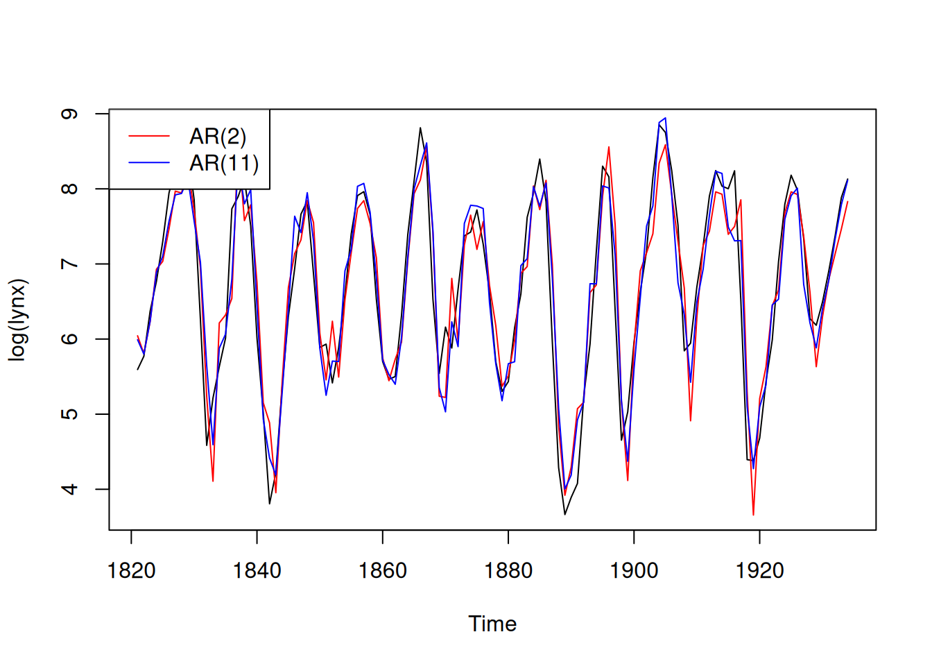
Compare quantile of measurement data with theoretical distribution
qqnorm(fit.2$residuals,main="Normal Q-Q Plot: AR(2)")
qqline(fit.2$residuals)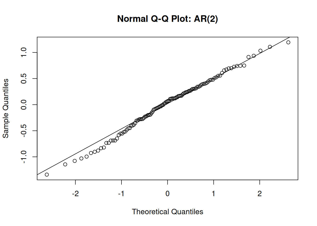
A moving average MA(q) model is a model in the form
\[ X_t = E_t + \beta_1 E_{t-1} + \beta_2 E_{t-2} + \dots + \beta_q E_{t-q} \]
with the time series \(E_t\) of innovations.
A moving average model does not have an explicit reference to previous values; only the innovation parts are considered.
set.seed(42)

#MA(2)
plot(arima.sim(n=100,list(ma=c(2,0.4))))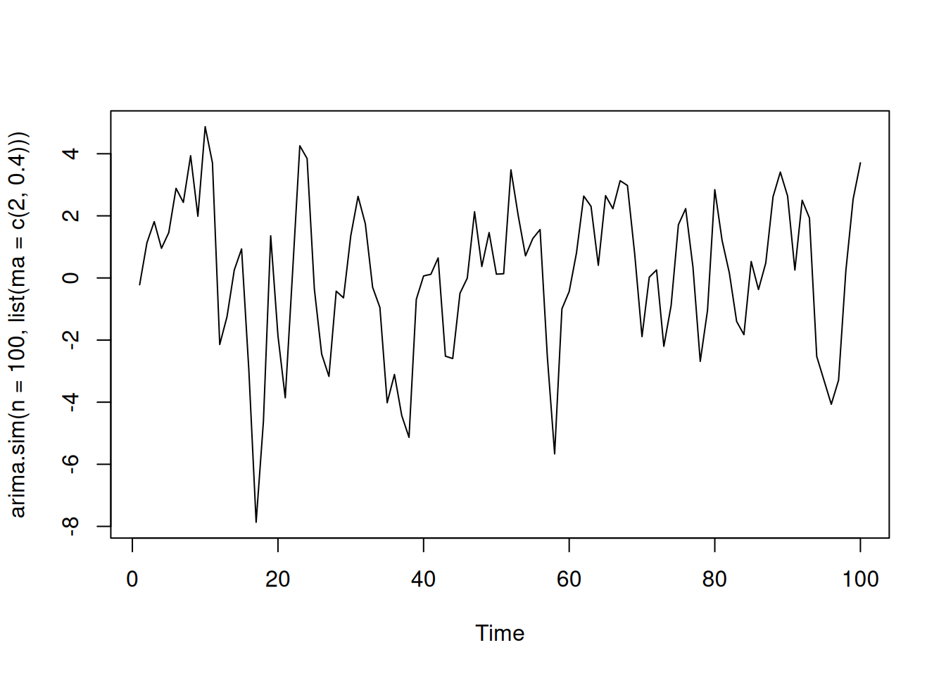
plot(ARMAacf(ma=c(2,0.4),lag.max=20),type="h",ylab="ACF")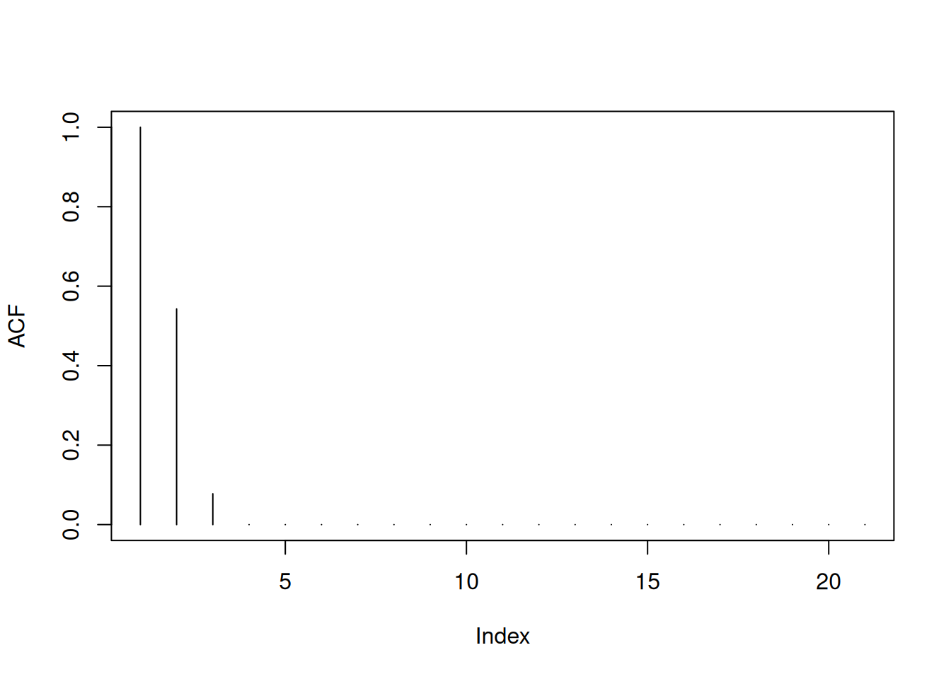
plot(ARMAacf(ma=c(2,0.4),pacf=T,lag.max=20),type="h",ylab="PACF")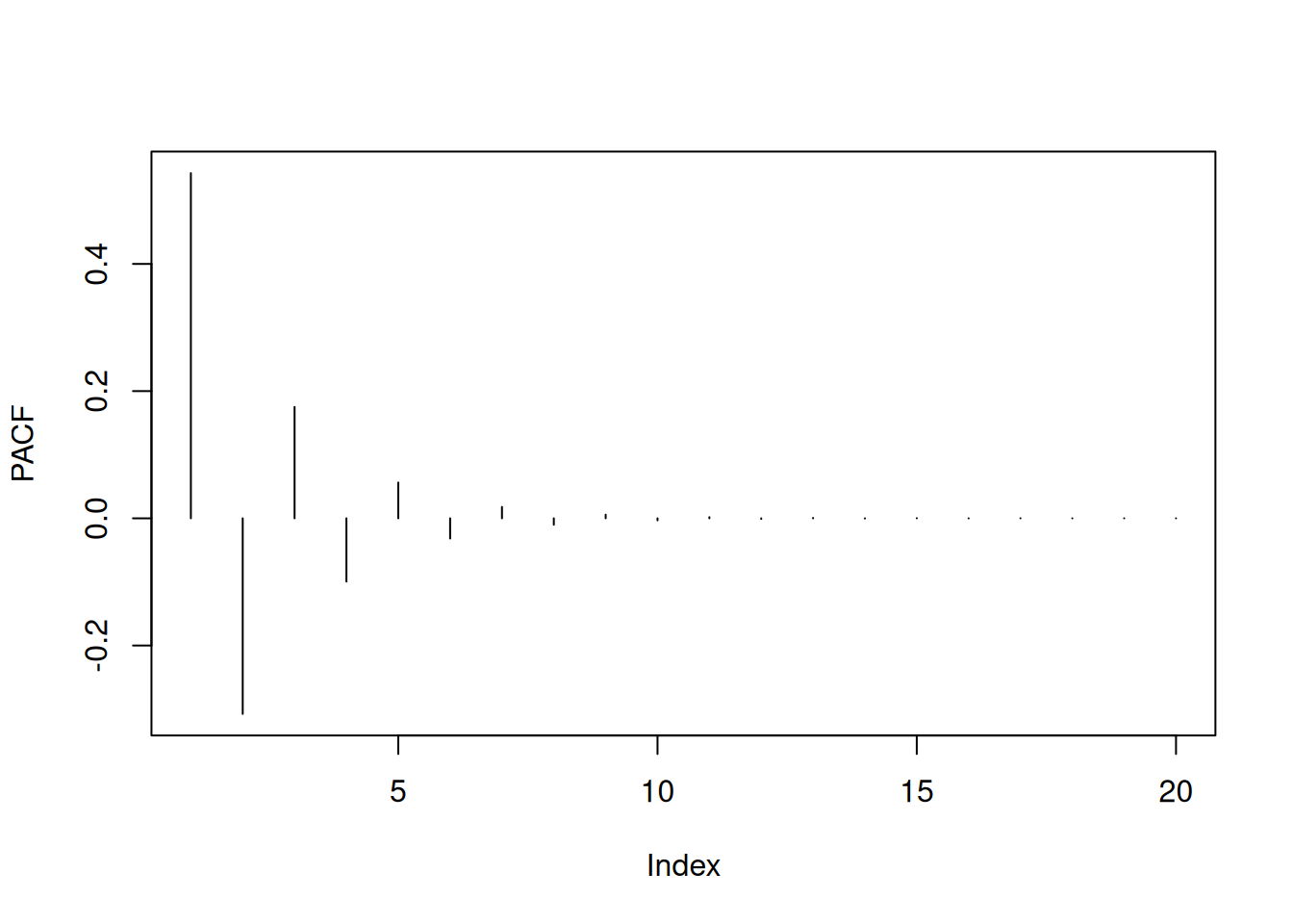
Generalization: In general, we can show that the autocorrelation function of an \(MA(q)\) vanishes for all lags larger than \(q\).